Some examples

For example, if you are interested in \(\bar{x}\), the mean number of hours that intro stat students sleep every night (using variable Sleep from the dataset students), the sample statistic would be:

mean(~Sleep, data=students, na.rm=TRUE)

## [1] 7.343511

(Note the “na.rm=TRUE” input - this tells R to ignore any missing values in the dataset when computing the mean. If you don’t include this input, then if there are missing values (NA) in the data, the result of your calculation will also be NA.)

Another example: what if you wanted to use the variable Rank in the students dataset to estimate \(\hat{p}_{oldest}\), the sample proportion of intro stat students who are oldest siblings?

prop(~Rank=='Oldest', data=students)

## prop_TRUE 
## 0.3435115

More advanced examples

More complicated sample statistics can also be computed. For example, what if the parameter of interest is the difference in mean GPAs (variable GPA) between intro stat students who plan to do further education after graduating from college, and those who plan to get jobs (variable Plans)?

We can compute the mean for both groups:

mean(~GPA | Plans, data=students)

##     Educ      Job 
## 3.447044 3.382988

Then we just need to take the difference between them – we can use the function diff() to do it.

diff(mean(~GPA | Plans, data=students))

##         Job 
## -0.06405607

Notice that the output is labelled Job. Which way did the subtraction happen?

We can also compute differences in proportions. For example, let’s find the difference in proportions male and female intro stat students who plan to get jobs after college graduation. First, we can make a table of the two relevant variables, Gender and Plans, using the input format='prop' to get the results as proportions rather than number of observations:

tally(~Plans | Gender, data=students, format='prop')

##       Gender
## Plans     Female      Male
##   Educ 0.2941176 0.3968254
##   Job  0.7058824 0.6031746

We need to isolate just the second row of the table:

tally(~Plans | Gender, data=students, format='prop')[2,]

##    Female      Male 
## 0.7058824 0.6031746

Then take the difference.

diff(tally(~Plans | Gender, data=students, format='prop')[2,])

##       Male 
## -0.1027077

The main idea

To get a bootstrap sampling distribution, we will follow the process:

1. Get a sample from the population (this is the dataset).
2. Resample “bootstrap samples” from the sample. Each one should be the same size as the original dataset, taken with replacement from the dataset.
3. Compute the sample statistic for every bootstrap sample.
4. The collection of many sample stats is the bootstrap sampling distibution (BSD). The standard deviation of the BSD is called the standard error.
5. Compute a confidence interval for the population parameter using the BSD.

To do this, we first have to think about how to take a single bootstrap sample from the data. We won’t have to do this step when using real data to compute a CI; we are just doing it here for illustration, to better understand how the resampling is done.

Examples

To get a bootstrap sample from a dataset, we will use the function sample. It has inputs size – here we want size to be the number of cases in the original dataset – and replace – we will use replace==TRUE to sample with replacement.

For example, to take one bootstrap sample from the students dataset, we would run the r code:

sample(students, size=nrow(students), replace=TRUE)

Note that no result will be printed to the screen when you run this code. It does work, though…

You try. How would you compute one bootstrap sample from the HELPrct dataset? *(If your code runs without an error, it’s probably correct…but nothing will print to the screen as a result. You can use the hints to check your work.)

sample(..., size=nrow(...), replace=TRUE)

sample(HELPrct, size=nrow(HELPrct), replace=TRUE)

Example

For every bootstrap sample, we will have to compute the sample statistic.

To do this, the code will be almost exactly the same as the code used to compute the sample statistic from the original dataset. The only difference is that instead of data=dataset.name, you will input data=sample(...) so that the data used for the calculation is a boostrap sample.

Here’s an example of computing the sample stat for one bootstrap sample, if the parameter of interest is the proportion intro stat students who are the youngest among their siblings:

prop(~Rank=='Youngest', 
     data=sample(students, size=nrow(students), replace=TRUE))

## prop_TRUE 
##  0.351145

Note: again, we won’t have to run this code as part of the final calculation of a bootstrap distribution. We are building up to the full code needed to compute the bootstrap distribution, and this is just one piece of it. Once you see how to do the whole thing, you don’t need to do this first anymore.

Practice

Compute the sample statistic for one bootstrap sample, if the parameter of interest in the proportion of intro stat students who are the oldest among their siblings.

prop(~..., data=sample(...))

prop(~Rank==..., 
     data=sample(..., size=nrow(...), replace=TRUE))

prop(~Rank=='Youngest', 
     data=sample(students, size=nrow(students), replace=TRUE))

What about the sample statistic for one bootstrap sample, if the parameter of interest is the difference in proportions male and female intro stat students who do exercise regularly?

diff(tally(...,...,...)[...])

diff(tally(~...|..., data=sample(...), format=...)[...,])

diff(tally(~Exercise|Gender, 
           data=sample(students, size=nrow(students), replace=TRUE),
           format='prop')[2,])

sample() method

We can compute a BSD for a proportion in a similar way. For example, a BSD for the proportion intro stat students that are male:

BSD <- do(1000)*prop(~Gender=='Male',
                     data=sample(students, size=nrow(students), replace=TRUE))
head(BSD)

Notice the somewhat strange variable name TRUE.…

shortcut rflip() method

There is another way (a bit of a shortcut) to find a bootstrap distribution that only works if the parameter of interest is one proportion. It uses the function rflip(), which flips and imaginary coin a certain number of times. You can specify the probability of getting “heads” on each imaginary coin-flip.

For the students data, the sample proportion Male from the real data was 0.48 and the size of the dataset was 131 observations:

prop(~Gender=='Male', data=students)

## prop_TRUE 
##  0.480916

nrow(students)

## [1] 131

So each bootstrap sample is like the outcome of a set of n=131 coin flips with probability of “heads” (Male), prob=0.48.

Thus, we can compute a bootstrap distribution via:

BSD <- do(1000)*rflip(n=131, prob=0.48)
head(BSD)

Your turn: try using rflip() to generate a bootstrap sampling distribution for the proportion intro stat students who plan to go on for further education after college graduation.

BSD <- do(...)*rflip(n=..., prob=...)

BSD <- do(1000)*rflip(n=nrow(students), 
                      prob=prop(~Plans=='Educ',data=students))

Example: BSD for difference in means

What about a bootstrap sampling distribution for the difference in mean GPA between students who plan to get a job after graduation, and those planning to do more schooling?

#sample stat
diff(mean(~GPA | Plans, data=students))

##         Job 
## -0.06405607

#BSD
BSD <- do(100)*diff(mean(~GPA | Plans,
                         data=sample(students,
                                     size=nrow(students), 
                                     replace=TRUE)))
head(BSD) #to see variable names in BSD dataset

gf_histogram(~Job, data=BSD)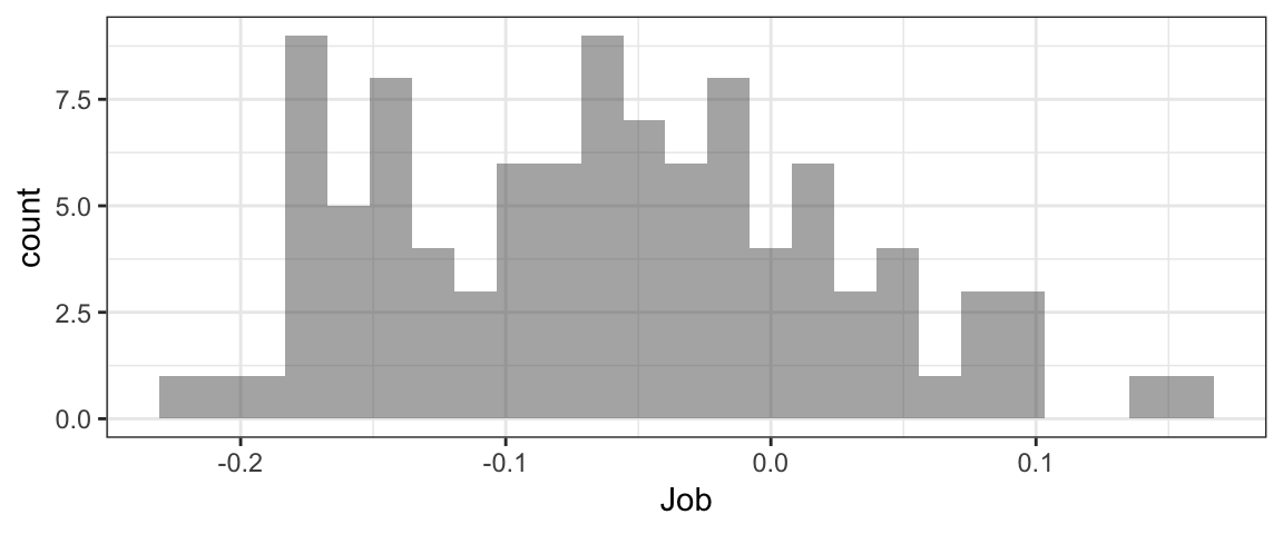

Example: BSD for difference in proportions

Similarly, we can find a BSD for a difference in proportions - for example, the difference in proportion students who exercise, between those planning to get a job after college and those planning to do more schooling.

#sample stat:
diff(tally(~Exercise | Plans, data=students,
           format='prop')[2,])

##         Job 
## -0.06950904

#bootstrap CI:
BSD <- do(100)*diff(tally(~Exercise | Plans,
                          data=sample(students,
                                      size=nrow(students), 
                                      replace=TRUE),
                          
           format='prop')[2,])
head(BSD) #to see variable names

gf_histogram(~Job, data=BSD, bins=10)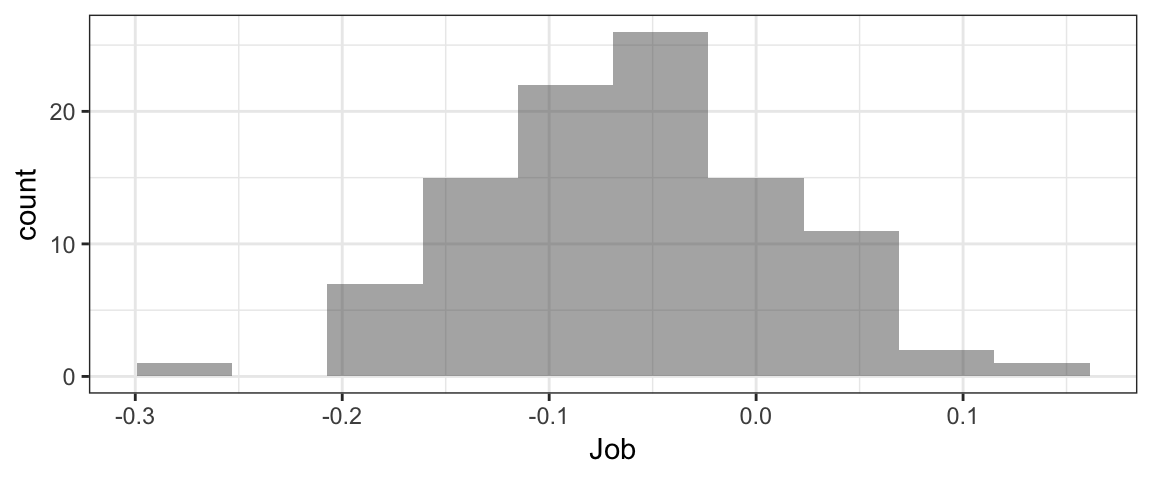

Your turn…

Try applying what you’ve learned so far to try a few more complex examples.

First, find a bootstrap sampling distribution for the difference in mean hours of sleep per night (variable Sleep) between students who exercise, and those who don’t (variable Exercise).

BSD <- diff(mean(...,data=...))

BSD <- diff(mean(...,data=sample(...)))

BSD <- do(1000)*diff(mean(~Sleep | Exercise, 
                 data=sample(students, size=nrow(students), replace=TRUE)))
head(BSD)

Now, try finding a BSD for the difference in proportion men and women who are oldest children:

BSD <- do(...)*diff(tally(..., data=..., format=...)[...])

BSD <- do(...)*diff(tally(~... | ..., data=sample(students, size=...), replace=TRUE), format='prop')[...,])

BSD <- do(1000)*diff(tally(~Rank | Gender, data=sample(students, size=nrow(students), replace=TRUE), format='prop')[2,])
head(BSD)