Halloween Candy Example

For example, let’s assume that the number of pieces of candy Grand Rapids kids get trick-or-treating on Halloween follows a normal distribution with mean 63 and standard deviation 21.

(Note: this is neither a test nor a CI; the distribution is not a bootstrap or randomization distribution. We are just claiming that the actual population distribution of candy-pieces-per-kid is Normal, as a simple first example…)

The distribution looks like this:

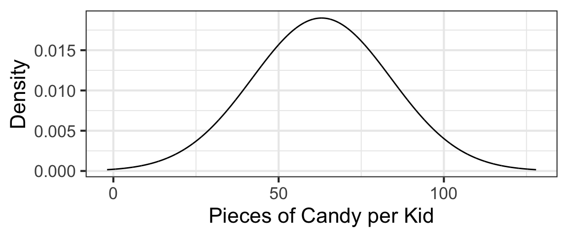
Given this scenario, what is the probability of a kid getting at least 100 pieces of candy? This probability corresponds to the area under the normal curve shown above, for x-values of 100 or greater:

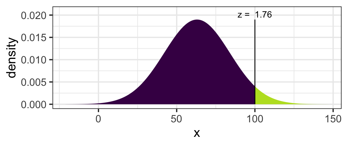
The probablity of getting at least 100 pieces is 0.04.

To compute this value with pnorm(), we need to tell R:

• What the value of interest is (100 pieces of candy)
• The mean of the relevant normal distribution (63 pieces)
• The standard deviation of the relevant normal distribution (21 pieces)
• Whether we want R to compute the area under the curve for less than the value of interest (input lower.tail=TRUE) or greater than the value of interest (input lower.tail=FALSE)

For example:

pnorm(100, mean=63, sd=21, lower.tail=FALSE)

## [1] 0.03904269

Halloween Candy Practice

Your turn: what is the probability of getting less than 50 pieces of candy, if the distribution of pieces of candy per kid follows a normal distribution with mean 63 and standard deviation 21? (Verify that the correct answer is 0.268.)

Another example

If the proportion Halloween candy secretly thrown out by parents follows a normal distribution with mean 0.40 and a standard deviation of 0.11, what is the probability of a kid’s parents throwing away at least 90% of her candy? (Verify that the probability is only about 0.0000027 - what a relief!)

Example Problem

For example, imagine we used the Zandee survey data to create a randomization distribution to test whether there is a difference, by neighborhood, in the proportion of people who have had a recent medical checkup.

Parameter and Sample Stat

The parameter of interest is \(p_{Heartside} - p_{Creston}\), the difference in proportion who’ve had a checkup, between neighborhoods. We can compute the corresponding sample statistic from the data.

tally(~checkup | neighborhood, data=zsurvey, format='prop')

##        neighborhood
## checkup   Creston Heartside
##     no  0.2981366 0.2704918
##     yes 0.7018634 0.7295082

s.stat <- diff(tally(~checkup | neighborhood, data=zsurvey, format='prop')[2,])
s.stat

##  Heartside 
## 0.02764484

Hypotheses

We want to test:

\[H_0: p_{Heartside} - p_{Creston} = 0\] \[H_A: p_{Heartside} - p_{Creston} \neq 0\]

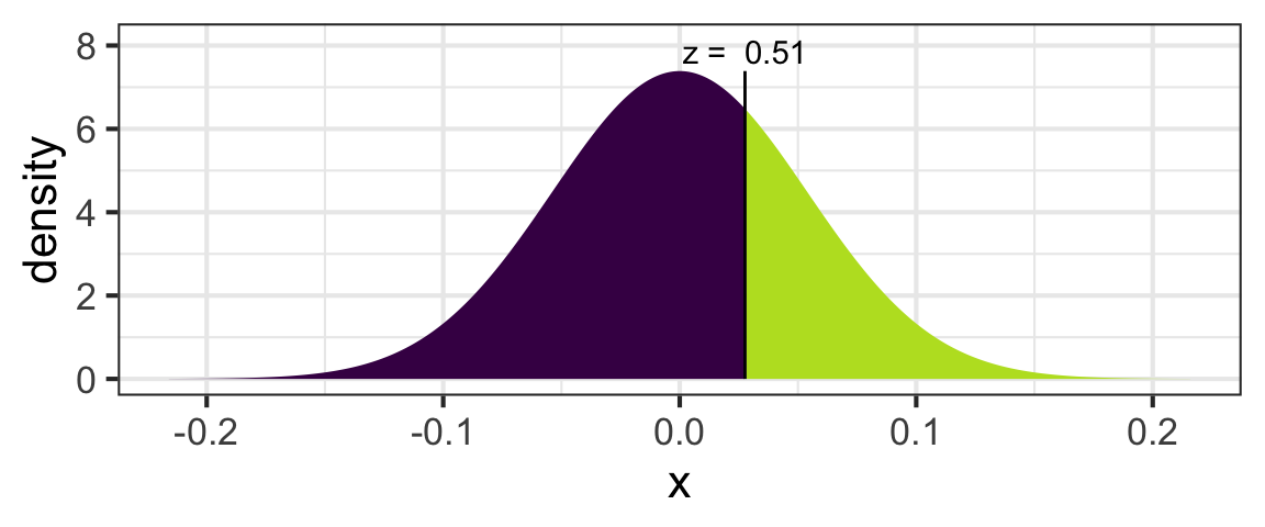
So our randomization distribution will be centered at the \(H_0\) parameter value, 0 (meaning there is no difference in proportion people who have had checkups between neighborhoods).

Imagine that the standard error of this randomization distribution was given to you: it is 0.054.

The figure below illustrates the randomization distribution, and the calculations related to finding the p-value of the test.

Using pnorm()

Now, use pnorm() to compute the p-value and verify that the correct p-value is 0.061. Recall: the parameter of interest is the difference in proportion people who have had checkups; the sample statistic is 0.0276, the \(H_0\) value is 0, and the SE of the randomization distribution is 0.054.

Another example

Imagine that a nonprofit in West Michigan provides a free ride program to provide transport to medical appointments. They have limited resources, so they only provide this service in areas where the proportion of people without access to rides is 75% or more. Should they start service in the Zandee study area?

We want to test:

\[ H_0: p = 0.20\] \[ H_1: p > 0.20\] The alternate is one-sided because the nonprofit only cares if the proportion without rides definitely exceeds 20%; if it is 20% or less, it’s all the same to them.

The sample proportion people without transport in the study area is 0.244. The SE of the relevant randomization distribution is 0.023. What is the p-value of the test? (Verify that the correct answer is 0.028.)

Example

For example, for the transport question, we found the p-value using the information:

• Sample stat: the observed proportion without transport is 0.244
• \(H_0\) value: the null hypothesis states that the true proportion without transport is 0.20.
• Standard error: the SE was given to us; it is 0.023.

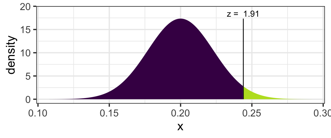
To compute the p-value with pnorm():

pnorm(0.244, mean=0.20, sd=0.023, lower.tail=FALSE)

## [1] 0.02787124

Alternatively, we could find the standardized test statistic. Confirm that the standardized test stat in this case is 1.913:

Now, find the p-value by comparing the standardized test statistic to a normal distribution with mean 0 and sd 1. We should again get a p-value of 0.028.

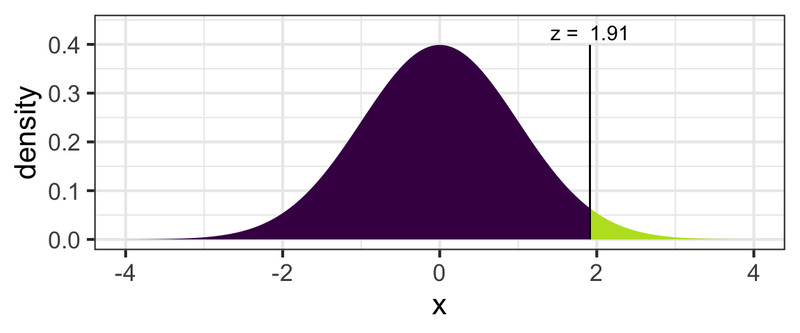
How would you compute this value using pnorm()?

pnorm(...,mean=,sd=,lower.tail=...)

Look back and verify: we got the same solution (p-value) by both methods!

Another example

Try another example. Verify that, for the other case study we tried, the standardized test statistic is 0.511 and the p-value is 0.609. Helpful information (from before) is repeated below.

• Parameter of interest: \(p_{Heartside} - p_{Creston}\)
• Sample statistic: 0.0276
• \(H_0: p_{Heartside} - p_{Creston} = 0\)
• Standard error of randomization distribution: 0.054